Prop Presentations for Linear Algebra: The $\mathbf{cb}_k$ Calculus

Overview

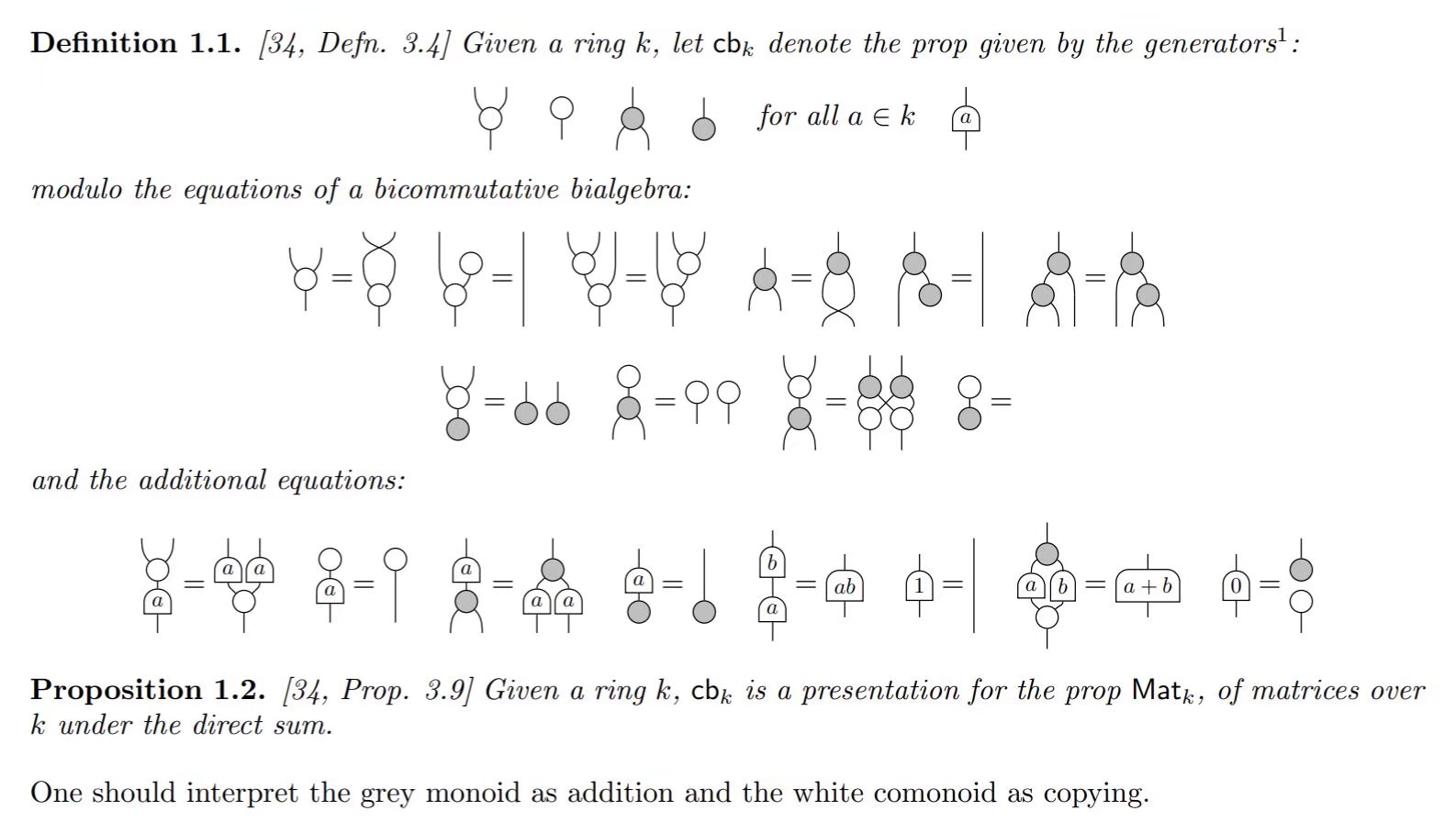
I have finally traced the definitive origin of this elegant piece of graphical mathematics by Dr. Peng! The fragment I was studying belongs to the seminal work "Graphical Linear Algebra" (specifically, see arXiv:2105.06244). This paper provides the rigorous categorical "source code" for representing linear algebra not through grids of numbers, but through the topology of string diagrams.

The specific formalism identified is the theory $\mathbf{cb}_k$ (standing for commutative bialgebra with scalars over a ring $k$). The central result is breathtaking in its simplicity and power: this diagrammatic language is a complete presentation for the prop $\mathbf{Mat}_k$. In other words, diagrams are matrices, and topological manipulation is linear algebra.

For those interested in a more pedagogical entry point, the authors maintain an incredible resource at graphicallinearalgebra.net, which unfolds this theory as a narrative about the interaction between two fundamental operations: Copying and Adding. Below is a detailed academic note synthesizing the formal definition from the paper with the intuitive insights from the website.

---

Academic Note: The Prop $\mathbf{cb}_k$ and Diagrammatic Reasoning

1. Introduction to the Formalism

The core idea is to define a Prop (Product and Permutation category)—a symmetric monoidal category where objects are natural numbers representing wire counts ($n, m, \dots$) and morphisms are diagrams mapping $n$ inputs to $m$ outputs.

The specific prop defined in the literature is $\mathbf{cb}_k$. It models the behavior of matrices over a ring $k$ equipped with the direct sum operation.

2. Generators: The Alphabet of Linear Algebra

According to Definition 1.1 (based on [34, Defn 3.4] in the source), the language is built from three distinct classes of generators.

(Note: In the diagrams below, time flows from bottom to top. Inputs are at the bottom, outputs are at the top.)

A. The Copying Structure (The "White" Comonoid) These generators form a commutative comonoid structure.

• The Copier ($\Delta$): A white node splitting 1 wire into 2.

  $$\begin{matrix} \mid & \mid \\ \nwarrow & \nearrow \\ & \circ & \\ & \mid & \end{matrix}$$
  • Semantics: This represents the linear map $V \to V \oplus V$ given by $v \mapsto (v, v)$. In the blog's terminology, this is the "Crema"—the ability to clone data.

• The Discarder/Counit ($\epsilon$): A white node terminating a wire.

  $$\begin{matrix} \circ \\ \mid \end{matrix}$$
  • Semantics: This is the map $V \to \{0\}$, effectively "deleting" a variable.

B. The Adding Structure (The "Grey" Monoid) These generators form a commutative monoid structure.

• The Adder ($\mu$): A grey (shaded) node merging 2 wires into 1.

  $$\begin{matrix} & \mid & \\ & \bullet & \\ \nearrow & & \nwarrow \\ \mid & & \mid \end{matrix}$$
  • Semantics: This represents the linear map $V \oplus V \to V$ given by $(u, v) \mapsto u + v$. The blog refers to this as "Zucchero"—combining resources.

• The Zero/Unit ($\eta$): A grey node starting a wire from nothing.

  $$\begin{matrix} \mid \\ \bullet \end{matrix}$$
  • Semantics: This injects the additive identity (0) into the wire ($k \to V$).

C. The Scalar Structure

• Scalar Multiplication: A box or bead labeled with $a \in k$. $$\begin{matrix} \mid \\ \boxed{a} \\ \mid \end{matrix}$$
  • Semantics: Represents the map $v \mapsto a \cdot v$.

---

3. The Equational Theory (Relations)

The power of $\mathbf{cb}_k$ comes from the rules governing how these nodes interact. The system is defined modulo the equations of a Bicommutative Bialgebra.

I. Monoid and Comonoid Laws

• Associativity (Grey): Connecting two Adders in sequence is equivalent regardless of grouping. $$\begin{matrix} \mid \\ \bullet \\ \nearrow \ \nwarrow \\ \mid \quad \ \bullet \\ \quad \ \nearrow \ \nwarrow \end{matrix} \quad = \quad \begin{matrix} \mid \\ \bullet \\ \nearrow \ \nwarrow \\ \bullet \quad \ \mid \\ \nearrow \ \nwarrow \quad \end{matrix}$$
• Co-associativity (White): The same law applies to the Copying structure (upside down).
• Commutativity: The Adder and Copier are symmetric; swapping input/output wires changes nothing.

II. The Bialgebra Law This is the most critical equation in the entire system. It defines how Addition and Copying interact. It asserts that copying the result of an addition is the same as adding the results of copies.

$$\text{Diagrammatically:}$$ $$\begin{matrix} \mid & & \mid \\ \nwarrow & & \nearrow \\ & \circ & \\ & \mid & \\ & \bullet & \\ \nearrow & & \nwarrow \\ \mid & & \mid \end{matrix} \quad = \quad \begin{matrix} & \mid & & \mid & \\ & \bullet & & \bullet & \\ \nearrow & & \times & & \nwarrow \\ & \circ & & \circ & \\ & \mid & & \mid & \end{matrix}$$

• Left Hand Side: Add two inputs ($\bullet$), then Copy the result ($\circ$).
• Right Hand Side: Copy both inputs first ($\circ \circ$), swap the inner wires ($\times$), and Add them separately ($\bullet \bullet$).

Algebraically, this enforces the distributive law: $\Delta(x + y) = \Delta(x) + \Delta(y)$

III. Scalar Relations The "Additional Equations" ensure the scalars behave as a Ring:

• Multiplication: Composing box $a$ and box $b$ equals box $ab$. $$\begin{matrix} \boxed{b} \\ \mid \\ \boxed{a} \end{matrix} \quad = \quad \begin{matrix} \boxed{ab} \end{matrix}$$
• Additivity: Parallel scalars summed together equal the scalar of the sum. $$\begin{matrix} \mid \\ \bullet \\ \nearrow \ \nwarrow \\ \boxed{a} \quad \boxed{b} \\ \nwarrow \ \nearrow \\ \circ \\ \mid \end{matrix} \quad = \quad \begin{matrix} \mid \\ \boxed{a+b} \\ \mid \end{matrix}$$
• Identity: A scalar box of $1$ is just a wire. A scalar box of $0$ is equivalent to Discarding then creating a Zero unit ($\epsilon$ followed by $\eta$).

---

4. The Main Result: Completeness

Proposition 1.2 [34, Prop. 3.9] states:

Given a ring $k$, $\mathbf{cb}_k$ is a presentation for the prop $\mathbf{Mat}_k$ of matrices over $k$ under the direct sum.

Interpretation: This is a Soundness and Completeness theorem.

1. Soundness: Every equation derivable in diagrams is a true statement about matrices.
2. Completeness: Every true statement about matrices can be proven using these diagrams.

There is an isomorphism of categories: $\mathbf{cb}_k \cong \mathbf{Mat}_k$ This transforms linear algebra from a theory of coordinates to a theory of connectivity.

---

Commentary: Methodology and Applications

Why Graphical Linear Algebra?

The transition from classical matrix notation ($A_{ij}$) to the $\mathbf{cb}_k$ calculus is analogous to the shift from assembly language to a high-level programming language.

1. Basis Independence: Classical linear algebra forces us to choose a basis immediately to write down a matrix. In $\mathbf{cb}_k$, we manipulate the linear maps directly via their structural properties (Copy/Add). We only "compile" to a matrix when absolutely necessary.

2. Topological Insight: Many properties of linear maps (like the trace, transpose, or feedback) are topological.

   • Transpose: Corresponds to rotating the diagram 180 degrees.
   • Trace: Corresponds to connecting an output wire back to an input wire (a loop).
   • Standard algebraic proofs involving indices ($\sum_k A_{ik}B_{kj}$) are notoriously error-prone. The diagrammatic proof is often a visual tautology—you simply "pull the wires straight."

3. Connection to Quantum Mechanics (ZX-Calculus): The structure of $\mathbf{cb}_k$ is strikingly similar to the ZX-calculus used in quantum computing. In ZX, we also have two colors (Green and Red spiders) that satisfy a bialgebra law.

   • In Linear Algebra ($\mathbf{cb}_k$): The structures are "Copy" ($\circ$) and "Add" ($\bullet$).
   • In Quantum (ZX): The structures correspond to complementary observables (Z and X bases). Mastering $\mathbf{cb}_k$ is an excellent prerequisite for understanding categorical quantum mechanics.

Applicability

This method is most effective when:

• Analyzing Large Networks: Signal flow graphs and electrical circuits are naturally modeled by these diagrams.
• Proving Structural Identities: When proving identities that hold for any dimension $n$, diagrams are superior to matrices, which often require fixing $n$.
• Tensor Networks: In machine learning and physics, the management of indices in tensor contractions is painful. Diagrammatic notation handles these contractions implicitly via wire connectivity.

References

• Primary Paper: Graphical Linear Algebra, arXiv:2105.06244.
• Original Definitions: Bonchi, Sobociński, Zanasi, Interacting Hopf Algebras, J. Pure Appl. Algebra (2014).
• Web Resource: Graphical Linear Algebra - A pedagogical blog by Pawel Sobocinski.